Probability density in phase space part 2: Detecting bifurcations

Continuing from last time.

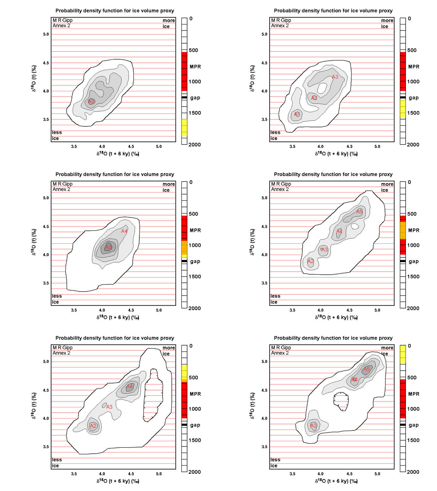
We can use a succession of probability density plots (PDPs) in sequence to show whether the number of Lyapunov Stable Areas (LSAs) changes, or whether the locations of individual LSAs moves. If the PDPs are displayed quickly enough, they may be displayed as a movie.

The significance of this is that a change in the distribution of LSAs may be indicative of a bifurcation in the system. A bifurcation is suggestive of a reorganization of the system, often appearing as a sudden response to a gradual change in one or more system parameters which has crossed some critical threshold.

Let's look at at the bifurcations in the global ice volume suggested by a sequence of PDPs from the past two million years approximately (original data from Shackleton et al., 1990).



There are a number of book-keeping details in this video. The sliding scale bar at the right shows the interval of time represented by each frame. There is a little black bar representing 30,000 years of missing data (that section of the core was badly undersampled.

The big red interval on the time bar labelled "MPR" represents the time of the "Mid Pleistocene Revolution" (also called the Mid-Pleistocene Transition) which represents a major change in the operation of the climate system.

The probability density of every frame was calculated on the basis of 270,000 years of data, so the blocks that include the undersampled bit actually represent the available data over an interval of 300,000 years. There is a possibility that some bias may have resulted.

As is normal for geological projections, the earliest PDP is presented first. The movie therefore flows forwards in time, and we see that in general, over the past 2 million years, ice volumes have increased (low ice volume is at lower left and higher ice volume is at upper right). The system has become more complex, as there are generally more stable zones in the later part of the record as opposed to the former.

Much of the complexity can only be appreciated by going back and looking at the actual state space superimposed on top of the probability density plot. One way of establishing the complexity of the climate system is by computing the complexity of the simplest epsilon machine that reproduces the patterns observed within the data (see also here--will do an entry on this at some point).

There is another abstract here which expresses the same ideas with different terminology.

Next in the series we will compare this method with alternate approaches taken from the literature.