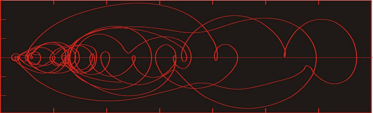
Dust flux, Vostok ice core

Dust flux, Vostok ice core
Two dimensional phase space reconstruction of dust flux from the Vostok core over the period 186-4 ka using the time derivative method. Dust flux on the x-axis, rate of change is on the y-axis. From Gipp (2001).

Tuesday, November 26, 2013

NRH gold deposits follow-up - still lots more gold out there!

Once again the good folks at Natural Resource Holdings (this time teamed up with Visual Capitalist) have updated their report (pdf) listing gold deposits greater than one million ounces in size.

In earlier postings I discussed briefly the expectations for the size-distribution of gold deposits, using an earlier list published by NRH and historical Nevada as examples. My conclusion was that the size-distribution of gold deposits follows a scaling law over at least a couple of orders of magnitude. There is a maximum size for gold deposits, because hydrothermal cells can likely only be so large before they become unstable and divide into smaller cells, leading to gold of one (natural deposit) being scattered over several discrete (economic) deposits. So how do we count them?

There are minimum sizes for deposits as well, primarily for economic reasons. So our scaling law only seems to be valid over a pretty limited range.


The yellow line is a possible scaling law to describe the size-distribution of gold deposits. Interestingly, its slope is 1 (pink noise), a very common scaling law in physical systems. It is quite different from the slope of 1.5 obtained from Nevada deposits. I'm not sure how to explain this, except that the Nevada deposits are almost exclusively of one type, whereas the global deposits represent all known settings.

As before, I don't expect that we will find many more huge (> 35 M oz) deposits; but there is potential to fill in the gap below the line in the 1 M oz range. From the above graph, we would still expect to find at least 400 more deposits, mostly in the 1 - 3 M oz range.

In reality, the number will likely be higher, as the census would still not be complete. It would be foolish to assume there are no deposits in Antarctica, for instance, even if climate and politics makes their exploitation unlikely. There are also numerous deposits on the seafloor, even if it may be a long time before control systems reach the point where they can correctly distinguish between ore and waste material while more than a km underwater.

All of this suggests that the yellow line needs to be shifted upwards--which opens up the possibility of many more deposits in the >10 M oz category still to be found. No guarantee on costs of all these, sorry.

---
Almost forgot to h/t Otto - although I'm sure I would have noticed this eventually.

Saturday, November 23, 2013

Interpretation of scaling laws for US income

It has been remarked that if one tells an economist that inequality has increased, the doctrinaire response is "So what?"
                                          - Oxford Handbook of Inequality

h/t Bruce Krasting

Social Security online has published a full report on income distribution in America.

Two years ago we looked at the distribution of wealth in America. Today we are looking at income.


There were a total of about 153 million wage earners in the US in 2012, which is why the graph suddenly terminates there.

As we have discussed before, in self-organizing systems, we expect the observations, when plotted on logarithmic axes, to lie on a straight line. Casual observation of the above graph shows a slight curve, which gives us some room for interpretation.

I have drawn two possible "ideal states"--the yellow line and the green line. Those who feel the yellow line best represents the "correct" wealth distribution in the US would argue that the discrepancy at the lower income (below about $100k per year) represents government redistribution of wealth from the pockets of the ultra-rich to those less deserving. Followers of the green line would argue the opposite--that the ultra-wealthy are earning roughly double what they should be based on the earnings at the lower end.

Which is it? Looking at the graph you can't tell. But suppose we look at the numbers. Adherents of the yellow line would say that roughly 130 million people are getting more than they should. The largest amount is about 40%, so if we assume that on average these 130 million folks are drawing 20% more than they should (thanks to enslavement of  the ultra-wealthy), we find that these excess drawings total in excess of $1 trillion. Thanks Pluto!

The trouble with this analysis is that the combined earnings of the ultra-wealthy--the top 100,000--earned a total of about $400 billion. They simply aren't rich enough to have provided the middle class with all that money.

Now let's consider the green line. Here we are suggesting that the ultra-wealthy are earning about twice as much as they should be, and let's hypothesize that this extra income is somehow transferred from the middle and lower classes.

As above, the total income of the ultra-rich is about $400 billion. If half of this has been skimmed from the aforementioned 130 million, they would each have to contribute about $1500.

I expect a heavier weight has fallen on those at the upper end of the middle-class spectrum; but even so, $1500 per wage earner does seem doable. Of the two interpretations, the green line looks to be at least plausible, and we are forced to conclude that those who believe the ultra-wealthy are drawing a good portion of their salaries from everyone else have a point.

But isn't $1500 per year a small price to pay to create a really wealthy super-class?

Paper on causes of income inequality full of economic axiomatic gibberish here (pdf).

Thursday, November 21, 2013

The Classification Problem

Posting has been light as I have been gobsmacked by something I discovered in a book that I've had for almost twenty years. I've always had trouble understanding it. I'm a geologist, and find this sort of thing (pdf) challenging.

It has to do with these probability density plots I've been making in phase space. I developed the idea intuitively, but the publishing has always been a slog because I had difficulty presenting a theoretical justification of my approach. I had made a leap of faith that each area of high probability density in phase space was centred about an attractor of indeterminate type.

It was a bit of a fluke getting the paper published in Paleoceanography--the reviewers weren't sure they agreed with it but were willing to give it a go. In terms of number of citations it ranks among the least influential publications in the journal's history.

The discovery was an interpretation of Zeeman's classification problem. His idea was that given a system which is described by a vector field on a manifold (say, a 2-d plane, which is what I have been using, but any surface is possible) so that the trajectory of the time-evolution of the system indicates a flow along the vectors; and given the system is somewhat noisy, so that there is a small random component to evolution along the trajectory; then the end-state of probability densities from all possible initial states on the manifold will be an invariant property of the vector field. What you will end up with will be diffuse balls of higher probability around each of the attractors on the manifold in phase space.

I read this as a justification of my intuitive approach, and he's a real mathematician.

Edit: Reference

Zeeman, E. C., 1988. Stability of dynamical systems. Nonlinearity, 1: 115. doi.org/10.1088/0951-7715/1/1/005

Saturday, November 16, 2013

Ode to Janet Yellen

The only problem with this song is that it should have been written in 1913.


Wednesday, November 13, 2013

Complexity, bifurcations, catastrophe

What makes a system complex?

It is a perplexing problem--both its description and its quantification. One might think that the description of a system as complex would suggest it has many subsystems each acting in accordance with its own rules, and interacting with each of the other subsystems in ways that we find difficult to describe. But there are systems involving very few "parts" which exhibit the kind of behaviour we call complex.

Another possible definition may stem from the notion of the compressibility of the system's information. Is it difficult to describe the sequential outputs in a manner that is simpler than merely listing all of our observations? A good random number generator would exhibit such behaviour, but we would not describe that as complex.

John Casti has proposed that the complexity of a system is at least partially dependent on the observer. He uses an example of a rock lying on the ground. To the layperson, there are only a limited number of ways to interact with the rock (kicking it, breaking it, throwing it, etc.) . To a trained geologist, there are more (as before, as well as mass-spectral geochem, x-radiography, electron probe, etc.). So the rock seems more complex to the geologist, but that additional complexity actually stems from the observer.

Another example can be share prices, where the complexity depends on the timing of your observations. If you look at the price of, say, Anadarko Petroleum over the past year, using closing prices only. (for disclosure--no position).


Then we can look at one-minute increments on a daily chart (Nov. 6, 2013).


Note that the variability within the two charts doesn't seem all that different despite the changes of scale. Lastly we could look at how trading in Anadarko looks over one second. One particular second, that is, between 3:59:59 and 4:00:00 on May 17 of this year.


You probably wouldn't expect a lot of change over 1 s, but in this case you would be wrong: the price fell from about $90 to $0.01 in less than 50 ms. That's a loss of $1 billion in market capitalization per millisecond--keep losing money at that rate and before long you're talking real money!

This all seems to trigger a philosophical debate--is the complexity present when none of the observers are capable of seeing it? In the case of Anadarko, if you were a pension fund, your losses would have been real (although the trades were all cancelled and reversed after market close).

If the complexity of a system arises from within, then what characteristics do we ascribe to complexity. One characteristic is discontinuous behaviour, particularly when the inputs to the system are continuous. For instance, tectonic processes gradually cause stresses to accumulate in an area in a fairly uniform fashion, until a critical threshold is reached and the earthquake occurs.

The branch of mathematics that investigates the sudden onset of convulsions wrought by a slow change is called catastrophe theory. Catastrophe theory is generally considered to be a branch of bifurcation theory. By bifurcation we normally mean some change in the operations of a complex system. It could represent a transition from one stable state to another. It could also represent the development of new areas of stability in phase space (or their disappearance) or simply a change in the nature of a chaotic attractor.

In particular, sometimes the sudden appearance of a new mode of stability is brought about by the changing value of a slowly migrating parameter past a critical threshold. Such behaviour is called a catastrophe, in the mathematical sense.

In the past few years we have seen a major change in the mode of operations in the markets. In particular, the rapid growth of high-frequency trading has added complexity at timescales where such behaviour did not previously exist. This is another example of a catastrophe.