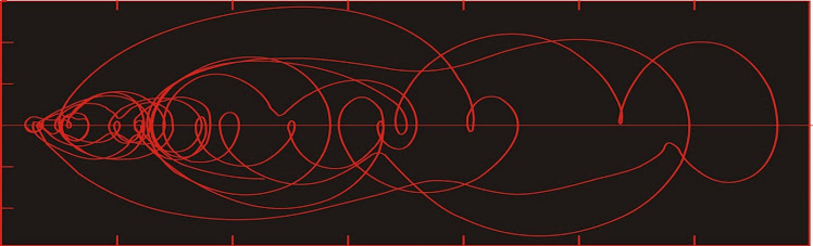
Dust flux, Vostok ice core

Dust flux, Vostok ice core
Two dimensional phase space reconstruction of dust flux from the Vostok core over the period 186-4 ka using the time derivative method. Dust flux on the x-axis, rate of change is on the y-axis. From Gipp (2001).

Thursday, June 30, 2011

Deconstructing algos, part 2: Leveraging chaos into high-frequency arbitrage opportunities

The recent elegant explanation for the activities of the HFT algos by Nanex seems likely to be a better one than the analysis that follows, as it answers the all-important question--why? In the following analysis we will look a little bit at how, but most or our interpretation of the results is coloured by the Nanex explanation. It explains why so many trades happen outside the bid-ask spread, particularly as the bid and ask prices are moving rapidly. They are scalping fractions of pennies from some poor fool who has data more than a few ms old.

As this is the reason, the method of choosing bid and ask prices pales in significance next to the methodology of stuffing the orders. This methodology I know nothing about and will not address. This article will address how to use this stuffing to create endless opportunities for arbitrage.

The principal advantage discussed in the Nanex report is stuffing the market with so many orders that competitors have trouble seeing the present state of the market. Whenever such inefficiencies are created, an arbitraging opportunity may also be created.

One method of creating arbitrage opportunities is through manipulation of time. We are accustomed to thinking of information flow as instantaneous, but it is limited by the speed of light. How might HFT take advantage of this?

Imagine for a moment that transatlantic communications were somehow extremely limited, so that a trader in New York could not see the present price of a stock in Paris, but would only see it after a two-hour delay. Any market participant who could somehow overcome this limitation would find a myriad of arbitrage opportunities.

Now look at the present. Let's suppose International Face Sucker (IFS) starts stuffing 100,000 bids per second into the pipe in New York. Let us say that those bids are x1, x2, x3, . . .

A market participant in Californa, Hedge Fool LLP (HF) is in the market and starts looking at the stream of bids coming down the pipe.

At 100,000 bids per second, the electronic signal only travels about  3 km between each bid. So at the time when HF sees the first bid (x1), and prepares its response (say, y1), IFS is actually sending quote x1500 into the dataverse. Where is the market? What is the current price?

Now suppose IFS has a branch in California. They have the same algo as IFS New York, and are running it so locally they observe x1 and HF's response y1--but they already know what x1500 is (or is that "is going to be"?), not to mention all of x2 through x1499. Might there be an arbitrage opportunity? Might there be 100,000 such opportunities every second?

A fraction of a penny 100,000 times a second--it isn't long before you're into real money.

Now IFS has branches in London, Paris, Sydney, Tokyo, Shanghai, Moscow--they are all running these arbitrage trades and who knows--maybe they are stuffing orders into their local bourses, using an algo known by all other branches and are arbitraging them as well.

The role of chaos

Not that it matters much, but what sort of algos are they using? I think they are mostly pretty simple.

The algo on the bizarre spreads seen here is straight forward, but hard to see how it profits.


As I've written elsewhere, the nat gas trading algo looked very similar to a simple chaotic function--the first such function ever identified.


Natural gas over a brief interval on June 8, 2011. Graph from Nanex.


 Nat gas price from above graph plotted against linear time.


Plot of first 5500 values for x using the Lorenz equation with parameters σ = 10, ρ = 24.7, β = 8/3.

You might think that using such a simple, well known function would mean that anyone could tag along for the ride. But you would be mistaken. Chaotic functions have a property called sensitivity to initial conditions, which makes them very useful in this particular application. Even in the unlikely event that some disgruntled former employee steals the software, its use will be extremely limited.

Note in the equations above we have three flow parameters, σ, ρ, and β, for which there are an unlimited number of choices resulting in chaotic behaviour of the overall function. In addition, we may choose any starting location, and we can also vary the time steps (basically x2 = x1 + time-step * dx/dt). Any arbitrarily small difference in any of the above parameters/variables leads to a dramatically different future evolution of the function. For instance, the two plots below (blue and red) are identical in all respects except for blue, σ = 10.01, and for red, σ = 10.00 (where only the red appears, the two curves are essentially identical).

The plot above represents about 16000 intervals, which could probably be squeezed into fewer than 5000 quotes, which IFS could blast out in maybe a twentieth of a second. If HF had stolen the program, and entered every parameter correctly, except for a typo ("10.01" instead of "10.00") then their estimate of the IFS bids will only be accurate for only about 25 ms. After that, HF might as well guess.

We could imagine IFS deciding on the next day's choice of parameters late in the evening, sending the numbers in an encrypted message to all their offices worldwide, and the next day they are all happily arbitraging away 100,000 times a second. They could change the parameters on an hourly basis--or every minute--it requires only a small amount of information to unspool an unlimited number of bids.

The only practical use for this software, if stolen, would be to use the same quote-stuffing method so your international subs could arbitrage the hell of the market. But that would be manipulation, if it falls into the wrong (read "your") hands. In the hands of IFS, of course, it is proper and judicious market management.

Monday, June 27, 2011

Nuclear power and geologic hazards 3: flooding

The two main considerations for impacts of geologic hazards are predictability and prevention. How predictable is the event, and what can you do to prevent damage to critical facilities. Most of the thinking about geological hazards (especially with respect to nuclear power plants) tends to centre around earthquakes, because they are difficult to predict, and because any prevention has to be designed into them, as there is normally insufficient warning to take any meaningful measures prior to an earthquake.

Two other kinds of hazard would be in this same category--volcanic eruptions and mass movements (landslides and sinkholes). However these are usually mitigated by avoidance. How many nuclear plants have you seen built on a volcano or on the side of a mountain? Sinkholes occur in particular geologic terrains, and (hopefully) power plants are not built on such ground.

Other natural hazards (hurricanes, flooding, forest fires) are not considered as serious because they are somewhat predictable and it is possible to mitigate damage immediately prior to the event.

Floods in particular are avoidable. I admit to a blind spot in thinking about the hazards of flooding affecting nuclear reactors because I assumed most were built in places where flooding doesn't happen (the tsunami affecting Fukushima being an unexpected event).

So why is there a reactor facing flood damage in Nebraska?

The buildings are designed to withstand floods up to a certain height. The forecast for the current flood on the Missouri River falls nearly 2 m short of this height, and so in principle, the reactor should be fine. On the other hand, after the events at Fukushima, people should be forgiven for regarding official pronouncements of reactor safety with a degree of skepticism.

The official report:

The 2,000-foot berm collapsed about 1:25 a.m. Sunday due to “onsite activities,” OPPD officials said. The Aqua Dam provided supplemental flood protection and was not required under NRC regulations. 

“We put up the aqua-berm as additional protection,” said OPPD spokesman Mike Jones. “(The plant) is in the same situation it would have been in if the berm had not been added. We're still within NRC regulations.”

The NRC says its inspectors were at the plant when the berm failed and have confirmed that the flooding has had no impact on the reactor shutdown cooling or the spent fuel pool cooling. 

The NRC said there is a separate, earthen berm to protect the electrical switchyard and a concrete barrier surrounding electrical transformers. 


Hmm, earthen berms. Let's see how they have held up historically against floods.


Here's a good-looking one. Mississippi River 1890. This is probably much like the one that just collapsed in Nebraska (minus all the black folks).


Here's another nice sturdy earthen wall (from an earlier edition of Keller's textbook). Wow, okay, maybe that's a bad example.


Here we go, this gorgeous berm built by (and photographed by) the US Army Corps of Engineers is just what we need to protect that power plant. Berms like it have made New Orleans completely invulnerable to flooding . . . err, ahem.

The trouble with earthen berms is that they tend to be reasonably strong against single events. But if flood waters pile up around them, the chance of failure through undermining increases dramatically. It is worse if the dam is subject to repeated floods. Was the berm and the ground beneath it checked for signs of water seepage after the last flood? Were any repairs necessary?

Individual owners of properties protected by berms are urged to inspect them every month. How likely is it that this has actually been done (rather than simply having had some paperwork filled out by a contractor)?

Earthen berms in Iowa have already suffered similar damage according to this news story.

What constitutes safety in design? Normally you look at building to withstand the events with recurrence intervals of 100 to 1000 years (the 100-year flood or 1000-year flood). The problems that many reactors in the US have is that the size of such events has recently increased (or rather the probability of occurrence of large-magnitude flooding event has increased markedly) due to urbanization and landscape changes (particularly the numbers of levees in upstream settings), and the power plants themselves have been called upon to serve much longer than their projected lifespans.

When you build a power plant that is intended to last 35 years, there is only about a 1-in-30 chance of a thousand year flood during its projected life. But when you now double that lifespan, and at the same time increase the size of the projected thousand-year flood, the likelihood that the plant will experience a flood beyond its design capabilities rises considerably.

Saturday, June 25, 2011

Big day

The last post appeared on Zero Hedge and there has been an incredible response.

I want to work out a couple of points here before replying on the Zerohedge board.

There was a post about me wanting the source code. It made me realize that I never said what it was I wanted to do.

What I am trying to do is put together a general approach to the forensic study of algorithmic trading. As in other forensic sciences, it would be nice to have a letter of confession from the perpetrator (read "source code")--but we cannot count on finding such a thing. What we can count on is the power of our own observations, our knowledge in applying some mathematical approaches, and our logical and/or intuitive approach to tying them together into what may evolve into a fruitful means of inquiry.

I do not represent that I know what I am doing. I do not know if what I am proposing will work. It is likely (perhaps most likely) that the methods of analysis proposed above will result in no useful conclusions, or worse--misleading conclusions.

I normally approach a scientific problem with a goal of testing a hypothesis. This problem is more like exploration--it is explored without clear hypotheses because I don't know what I may find. What would I have to see to convince me that the algorithms are manipulative rather than competitive? I don't know. I am merely hopeful that I will see something.

One poster commented that I would like to find evidence of manipulation so that I too could be ignored by the SEC. That seems to be close to the truth, and the outcome (if I did find such evidence) seems a little too likely to be funny. But even if I am to be ignored by the SEC, my thinking is that it is better to know than not to. Through knowledge there may be a chance at some kind of action--perhaps by people like us, if not the authorities.

Many comments have been constructive, offering other lines of potential inquiry. I thank you all for them. Some comments have not been--but that tends to happen whenever there is an element of anonymity. I see the importance of not taking it personally.

Friday, June 24, 2011

Deconstructing algos, part 1

The third part of the series on information theoretic methods of analysis for dynamic systems is taking longer than anticipated. Crunching the numbers is killing me. So I'll take a break from it and look a little farther forward--how we can use the methods I have been describing so far to forensically examine the algorithms used in various high-frequency trading events of the recent past.

As seen on Nanex and Zero Hedge, there has recently been a lot of strange, algorithmically driven behaviour in the pricing of natural gas and individual stock prices on very short time frames. In an earlier article I pointed out that the apparent simple chaos we observe in the natural gas price appeared to be an emergent property of at least two duelling algorithms.

In this series of articles we will begin analysis of the algorithms involved. Today's discussion will mostly focus on framing the issues that must be addressed in order to study unknown algorithms on the basis of their time-varying outputs. Future articles will present results from the various analyses.

We begin by looking at the activity in the natural gas price on June 8, 2011:


Let us also consider the pricing action in CNTY on June 21, 2011:


In both of these examples (many more such examples exist) there are three time series of interest to us--the bid price, the ask price, and the prices of trades. Additional information which may also be of use are such things as volume, size of bids, size of asks, and so on. In principal both the bid and ask prices form continuous series which are prone to instantaneous changes. The actual trades form a discontinuous time series with obsrevations at irregular intervals.

We don't have access to the code involved in these algorithms--nevertheless, we can learn something about the computational processes involved, within certain limitations. Unfortunately, just as is the case in studying time series recorded in rocks, we have to make some assumptions, and the validity of our assumptions goes a long way towards predicting the success of our endeavours.

Our first assumption is that the bid price and the ask price are being set by competing interests. This assumption is extremely important. It is possible that the bid and the ask are both being set by a single entity, or by two closely related entities who are using them to manipulate the natural gas price. We will go though in some detail the reasoning behind our assumption that there are competing interests involved below.

Secondly, we are approaching this problem assuming that prices are set and changed discontinuously in time rather than continuously in time. Subtleties of this assumption are discussed in the introduction of Bosi and Ragot (2010).

The methodologies we will explore are as follows:

Cross-correlation of the bid and ask series over selected windows. We choose limited time intervals rather than the entire record because we expect that each series will sometimes lead and sometimes follow. Peaks here will show whether one of the series leads or trails the other consistently or whether each one leads intermittently, which would support the idea that these are distinct dueling algorithms. It seems likely that the bid price will lead as both are declining, and the ask will lead as both are climbing. We should test this hypothesis.

One goal of this analysis will be to see if we can detect trigger points, where one stops following and begins leading. We will locate the times and see if the trigger can be identified, which is only likely if the trigger is some change in either price series, the price of a trade, the volume of a trade. Unfortunately, many other triggers are possible, and it may not be possible to identify them if they are, for instance, a random number generator seeded by, say, the thousandths-of-a-second digit at the instant of some distant event like the first pitch of a Yankee's game or when the secretary in the front office misspells 'the'.

Phase space reconstruction--the relevant time series (bid prices, ask prices, trade prices) each represent one-dimensional data sets. If the algorithms used can be visualized in higher-dimensional phase space, we may be able to reconstruct the overall architecture.

The advantage of this approach is that in principle the dynamics of the system will be contained no matter which output of the model we use. We only have measurements of the bid price, but have no idea what other outputs are generated by the same algorithm, even if these unknown outputs are critical to the decision-making module of the algo. The reconstructed phase space

The difficulties here are that 1) the function may change from leader to follower so quickly that the resulting trajectory through phase space is too short to interpret; 2) there may be multiple players on both the bid and ask, meaning the reconstructed trajectory through phase space is an amalgamation of two or more different functions, the instant of joining of which may be impossible to determine; and 3) it may prove impossible to properly define windows for the data, again creating an amalgamation in phases space of two or more different functions.

Epsilon machine reconstruction--We will need to try to identify the actual "work" done by these programs. How do they decide on a price? How do they "decide" to drop or raise their offer? Do they change? How are we to recognize when an algorithm changes its behaviour when all we have to deal with is the output? Can we recognize when the structure of the computation involved in the decision-making part of the algorithm changes, given our extremely limited knowledge of that structure?

These questions may be addressed using the ε-machine reconstruction approach suggested by Crutchfield (1994). The objective of this approach is to use an open-ended modeling scheme to describe the computational structure objectively, so that different practitioners working on the same data will come up with similar (hopefully identical) constructs. By encouraging an heirarchical architecture of undefined complexity, the method allows investigators to identify changes in behaviour of the the system.

This particular approach is built around discrete computation, so is amenable to data which are discrete rather than continuous in time. We assume that the discrete outputs (the time series, or stream of values) is the result of a computational process which is knowable. The data have to be organized, and (this is the key) repeated states are identified. It is possible that these states will be identified from the reconstructed phase space portraits above; alternatively they may be be defined by particular observations. These states may be identified as key strings of data, or may be recognized in complex functions by reconstructing the state space in a higher dimension. The ordering of the states is significant, as the state that appears first before another particular state is referred to as the predictive state, and the following state is the successor state.

The ε-machine is constructed by identifying all the predictive and successor states and  calculating the probabilities of all of their observed relationships. If more than one ε-machine is inferred, the sequence of these first-order ε-machines can be used to build a higher-order ε-machine. Given sufficient data, you may construct ε-machines of arbitrary order.


Information theory--as seen in recent articles, information theory may be used to characterize the complexity of the ε-machine reconstruction and the probability density. The yet-to-be completed third part of that series concerns methods of using information theory to find the optimum window length for creating a probability density plot of the reconstructed phase space. The subsequent parts of this series will concern itself with the analyses described above on the nat gas and CNTY algos, as well as others as they are found.

Given the limitations of time and computing resources, I can't guarantee a timeline. I regret that my speed of analysis is six or seven orders of magnitude slower than the incidents in real time.

Friday, June 17, 2011

Information theoretic approaches to characterizing complex systems, part 2: complexity of climate proxy data from probability density plots in state space

Last time the World Complex applied simple information theory to the probabilities of particular state transitions within the constructed epsilon machine representations of paleoclimate proxies.

Probability density is calculated by the method outlined here, and below, we see one frame of data for the oceanographic condition proxy (mid-ocean d13-C variability). In essence, the data are unfolded into two dimensions using the time delay method of phase space reconstruction. The probability density is estimated by mapping out a set of overlapping boxes through phase space, and the amount of time the reconstructed state lies within each box is calculated over a window (I have used 270-thousand-year windows--your mileage may vary). Similar windows have been created at 30 thousand year intervals going back nearly two million years.


The entropy of this distribution of data is calculated by reducing the number in each cell in the array above to a probability (a fraction of 270 thousand year duration). In the calculation of the above array, each observation is slotted into four separate cells, so the total "probabilities" add up to 4. The ideal correction would be to count up one cell in every four. What works as well is to use p(i) = t(i)/270,000, where t(i) are the elements of the array, sum up [-Σp(i)log p(i)]  for all non-zero terms and divide the total by four.


Calculating entropy for all windows for the oceanographic condition proxy and plotting the results below . . .


Higher values indicate higher entropy, which we normally equate with greater complexity. Oceanographic changes were highly complex in the early Quaternary (until about 1150 thousand years ago); but complexity fell through the middle Quaternary, reaching a minimum at about 750 thousand years ago); increased until 
about 450 thousand years ago, and has generally declined since.

I should point out here that when we average data over a window (say from 0-270 thousand years ago), the standard is to plot the result at the midpoint of the window (i.e., 135 thousand years ago). When you look at a plot of the 200-day moving average for a stock price, they plot that average at the end of the window, rather than the middle. This is an important difference.


If we consider individual probability density plots, we see that the area of phase space occupied by the attractor over the Quaternary has varied, but is generally about the same size at different times. We shall see below that this is not the case for the ice volume proxy and the paleomonsoon strength proxy.


The variation of complexity in the ice volume proxy phase space reconstruction with time is as follows:


There is a marked increase in complexity from the Early Quaternary (right side of the graph) to the Late Quaternary (left side of the graph). That complexity has dropped rather sharply in the most recent windows, and this last bit of variability appears to exceed the variability within the graph. Is this an indication we are on the cusp or a major change to the global climate system? 


The variation in complexity for the paleomonsoon proxy over the past 2 million years is as follows:


Once again there is a significant increase in complexity in the behaviour of the phase space portrait of the paleomonsoon strength proxy throughout the Quaternary. In the early Quarternary the behaviour of the system is quite simple, and is dominated by tight orbits around a single area of high probability. Complexity is much higher in the late Quaternary, but does fall off somewhat fairly recently.


Probability density plot for phase space portrait of paleomonsoon strength proxy, 
over a window from 1421 to 1691 thousand years ago.


Probability density plot for phase space portrait of paleomonsoon strength proxy,
from 281 to 551 thousand years ago. The larger number of LSA areas (high probability)
suggests greater complexity of behaviour in the Late Quaternary.


The overall picture of complexity through the Quaternary is in accordance with that inferred from the epsilon machine computation of our last installment.