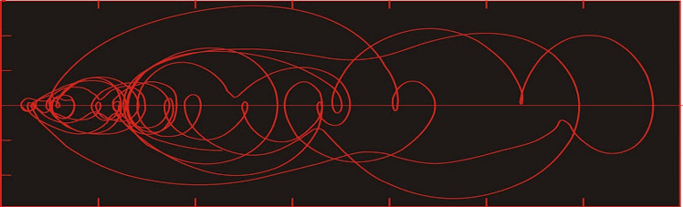
Dust flux, Vostok ice core

Dust flux, Vostok ice core
Two dimensional phase space reconstruction of dust flux from the Vostok core over the period 186-4 ka using the time derivative method. Dust flux on the x-axis, rate of change is on the y-axis. From Gipp (2001).

Wednesday, September 8, 2010

How Life Imitates the Stock Market, part 6: Clarifying phase space reconstructions

I will look at one approach for clarifying the phase space portraits we have constructed last time.

This approach is choosing a suitable embedding dimension, which is the number of dimensions of state space into which we will unfold our time series.

Embedding dimension

The curves in the reconstructed phase space should not intersect, if they are unfolded in the correct number of dimensions. The reason for this will become plain if we once again consider the reconstruction in terms of a function and all of its various time derivatives. Suppose that a system is completely described in a state space. These dimensions will be the scalar measurement, its first, second, and higher time derivatives (speed, acceleration, jerk, jounce or snap, etc.--in the scalar sense).

Each state is defined by a "position" in phase space, with coordinates being the scalar value, the rate of change, the second time derivative, etc.). At the next time step, a new state, with a "position" defined by a scalar, a time derivative, a second derivative, etc. each of which are uniquely defined from the previous state and the length of the time step.

For two different trajectories to intersect, the state at the point of intersection must define two alternative future states. But this is clearly impossible if the scalar and all of its time derivatives are identical. Thus, the best you can do is have two different trajectories approach arbitrarily closely. If I recall correctly, this argument was first proposed by Hirsh and Smale (1974).

One of the features looked for in a phase space portrait is groups of points on different trajectories which closely approach one another. In particular, we may find that there are regions of phase space towards which many different trajectories evolve, and these trajectories may each remain in one of these regions for some considerable time. Such regions may imply the existence of relatively stable (or metastable) states in the system, which is a possible predictor for future evolution of the system.

In order to determine whether such areas exist, we need to know if these neighbouring points on different trajectories are actually close to one another, or merely appear to do so because of the projection of our phase space.

Here we see hypothetical two-dimensional and three-dimensional portraits of the same system. In the two dimensional portrait, points A and B appear to be quite close.

In the three-dimensional phase space, we see that A and B are not close neighbours after all. If we made our interpretation on the basis of the two dimensional portrait, we would be in error.


In the diagram at left, points A and B are called false nearest neighbours. The presence of false nearest neighbours indicates that the state space is not defined in a sufficient number of dimensions (we would say that the embedding dimension is insufficient).

One therefore finds the embedding dimension by increasing the number of dimensions of our reconstructed phase space until there are no more false near neighbours.

The magnitude of the embedding dimension gives you an idea of the number of invariant parameters in the system--at least in an ideal world. Unfortunately, in the real world there is this thing called noise, which is infinitely dimensional; consequently ever higher-dimensional reconstructions reveal increasing numbers of spurious near neighbours which are demonstrated to be false in a higher dimension. One never reaches the point of having no false near neighbours.

So one may end up selecting an embedding dimension that seems reasonable. The estimate may be wrong, but can be assessed to a certain extent by studying closely the trajectories in higher dimensions using  mathematical methods to laborious to discuss at this time.

I will discuss the use of probability density in phase space next time.


Hirsch, M. W. and S. Smale, 1974. Differential Equations, Dynamical Systems and Linear Algebra, Academic, San Diego, Calif., 1974.

Wednesday, September 1, 2010

How life imitates the stock market, part 5: Choosing a lag for phase space reconstruction

We continue with reconstructing a phase space for Detour Gold Corp. (DGC-T). Disclosure -- long position (which long predates my use of this analytical tool).

A two-dimensional phase space can be reconstructed from a time series by creating a scatter plot of the time series against a lagged copy of itself. By doing so we create a plot which is topologically equivalent (though not absolutely identical to) a phase space consisting of the time series plotted against its first time derivative.

How much of a lag should we choose. It should be intuitively obvious that the lag should not be too small. If, for instance, we had pricing data for our stock that was collected at one-second intervals, a lag of 1 s would probably not show very interesting dynamics, as 1 s is not enough time for much to happen with price (except very rarely).

The price data in the DGC pricing time series is at one-day intervals, so that one day should be the smallest lag we can look at. Well, we could look at a zero lag plot, but it is not very interesting.

The zero-lag 2-d phase space for Detour Gold. Actually, it does show something interesting--there is something of a gap in price from about $25 to $27 and $28 to $29. But we could have learned that from a simple one-dimensional plot.

A lag of one day (for instance plotting Friday's closing price against Thursday's, etc.) looks a little more interesting. . .


It is a little difficult to make out where the graph starts, but its ending stands out, with the last price in our time series being just above $31. Here is the phase space with a lag of two days . . .


Many of the same features are present, but the curve diverges a little more from the diagonal line. Even though equivalent features can be found in both of the lagged time series, the specific shape of corresponding features changes somewhat from one lag to another.

Here is the phase space with a lag of three days.


And for four . . .


Nothing much new here. The overall form is the same, however you may notice that the lower part of the plot is spread away from the diagonal more than is the case in the one-day-lag phase space. The last plot also is not quite as tangled as the one-day-lag phase space.

Overall, this is not a very interesting plot. Part of it is because the dynamics of the stock performance over the last nine months has not been very interesting--at least from a dynamics perspective (it is always interesting to see a stock for which one has a long position rising).

The reason for the minor differences in the reconstructed phase spaces has to do with the connection between the lag, and the portion of the curve over which the slope (the first derivative) is calculated. When we used the price difference last time, we were actually using that as an estimate of the slope of the tangent to the price function. When I chose to take the price difference over a two-day period (and then divided by two), I was estimating the tangent slope from two points that were separated by two days.

In the small diagram at left, we are interested in finding the slope of the tangent (yellow line) to the curve at point T.

By using the price difference over two days, we calculate the slope of the green line segment, which is our estimate of the slope of the yellow line.

Because the only data we actually have are represented by the red blobs, we cannon find the slope of the yellow line directly.

The lag plot essentially estimates the slope of the yellow line differently.

For the one-day lag, your estimate of the slope is the short red line segment; for the two-day lag, the orange segment; three-day lag, the green; and for the four day lag, the estimate for the slope of the yellow tangent line is the slope of the blue segment.

Clearly, none of these look like particularly good estimates. So what is the relative merit of choosing one lag over another.

If the time series is especially busy, with a lot of variability, then the slopes estimated between neighbouring points will similarly show a lot of variability. If the the slopes are estimated between points that are farther apart (longer lag), there will be less variability.

The choice of a lag can therefore be influenced by the scale of the dynamics of interest. If you are interested in short timescale dynamics, you need to use a short lag, and if you are interested in longer-term dynamics, you need to use a longer lag.

The formal rules (first minimum of the average mutual information) is selected because this maximizes the differences between the two axes so that the maximum information is revealed.

Unfortunately, the DGC plots don't show a lot of interpretable dynamics. So let's look at some functions with some interesting dynamics.

The plot at left shows the plot of the proxy function for global ice volume over the past million years. Data from Shackleton et al. (1990).

In various papers and presentations over the past ten years I have used this record and others to study global climate dynamics.

The2-d state space reconstructed below used a lag of 6,000 years and covers about half of the record shown above (from 500,000 years ago until present).

Now here we have a phase space which allows us to interpret a lot about the dynamics of the system. It is a little complex, and like other plots above, it just consists of numerous clockwise loops overlapping each other.

The record would look better rendered in three dimensions, as the apparent intersections would be shown to be areas where the function passes beneath itself.

In the coming discussions we will look at ways to clarify the plot at left and see what can be interpreted from it.


Reference:

Shackleton N J, Berger A, Peltier W R. An alternative astronomical calibration of the lower Pleistocene timescale based on ODP Site 677. Trans R Soc. Edinburgh Earth Sci, 1990, 81: 251―261.

Saturday, August 28, 2010

How life imitates the stock market, part 4; reconstructing phase space portraits

Here is the price chart for the last nine months for Detour Corp (DGC-T) [Disclosure: long]

Now suppose we decide we want to know something about what is driving the price of this stock. We have a time series (here we've plotted the daily closing prices for the last nine months or so). We think the dynamics of this time series might be interesting and are hopeful that if we were to learn something of them it might help us decide when or at what price we would wish to buy (or sell) this stock.

We know very little about what drives stock prices. If we were to guess at a conceptual model for the dynamics governing this particular stock price, it would probably include: the gold price; the perception of expected expenses in developing the property; the perception of political problems (native concerns or sudden mining tariffs, or somesuch); or the general perception of the overall stock market.

A sophisticated observer might want to add some stochastic element as well as something that takes into consideration the psychology of the observers interested in this particular stock. For we often observe that stock prices have a sort of momentum--when they have been stuck in a narrow range for some time, they are more likely to remain within that range, but if they break decisively, the stock price can be driven by "momentum", whether such momentum arises from investor herding or confirmation bias.

The tripping of a psychological switch allows for the prospect of some sort of feedback within our pricing system. All in all, it is beginning to look like the differential equations used to describe our system are going to end up being at least in part nonlinear. And the time series outputs from nonlinear systems are notoriously difficult to understand (or model).

So our system is affected by numeous factors, all of which we would like to at least have the potential to analyze. But all we have is price. Is it enough? Many commentators (this is not intended to endorse the services of the linked gentlemen) tell us all we have to do is watch price. But are they right?

It turns out that they are. I know, I can hardly believe it myself. I must admit I have some doubts about whether these commentators understand why price is all that matters, but also acknowledge that once you have an empirical  method that works for you, you may not feel you need to understand why it works. In fact developing such an understanding may only subtract from the amount of time you have to make money.

The reason why price is all you need is one of the deep mysteries of ergodic theory. In short, all information concerning the dynamics of all the inputs is recorded in all of the outputs of a system. Price is just such an output. Equally well, you might use volume or change in price, as these will both reflect the dynamics in which we are interested; however the relative weights of each component driving the changes in price may be different for each of these time series. But the information is all present in each series, so we should not gain very much by studying price in conjunction with one of these other variables.

Now the dynamics of numerous different factors are not revealed within a one-dimensional plot, which is all the above chart really is. We have stretched out time, but had we not done so, we would have ended up with something like this.

Not much to see here. All you could really make out is the highest price (the top of the line) and the lowest price (the bottom of the line)

In order to see all the dynamics of interest, we need to "unfold" the plot of the time series into a phase space plot with enough dimensions to reveal all the dynamics of all the factors influencing it. Normally you will need at least three dimensions to really see anything interesting. More practically, the plot should never intersect itself.

One way of unfolding the data is to plot it against some other data series which is related somehow, but which can be considered independent. By this I don't mean looking at parallel line charts--I mean a scatter plot of one variable against another.

For paleoclimate studies you might plot your proxy data for global ice volume against, say, your proxy for atmospheric CO2 and/or your proxy for deep ocean temperature (e.g., Saltzman and Verbitsky, 1995).

We don't have so many variables to choose from, so let's look at the closing price plotted against daily volume for DGC. One advantage we have over the paleoclimatologists is that by definition, both of these data series are sampled at the same intervals, and we can obtain both series over the complete interval of study (the last nine months here). You won't believe how much of a problem this can be in studying natural time series.

To create the graph at right, I have plotted the daily closing price against the daily volume for each day over the last nine months. The points are plotted in chronological order, and a curved line (as per tradition) is drawn through the points.

Each plotted point is called a state, and the graph itself is called a state space (alternatively phase space is also used). The curved line represents the trajectory of the system as it evolves through time.

What we have here is a state space of sequential price-volume states for Detour Gold Corp. from late November 2009 to late August 2010.

The beginning of the plot is somewhere in the tangle near $15. There is so much action there it is hard to see. The end of the plot is easier to see--it is the tail of the graph there at middling volume and a price over $30. Interesting, but hard to interpret.

I could easily choose another data series to plot against price. This time I will plot daily price against the change in price from the previous close.

Here we actually have a plot that is easier to follow. Even though the beginning is hard to make out, there is little doubt about which way the system is evolving.

It is always moving clockwise around the loops, for the simple reason that below the horizontal axis, the price change was negative, meaning that the subsequent price is lower than the previous price.

Above the horizontal axis, the price change is positive, so the subsequent price must be higher than the previous price.

The further the curve is from the horizontal axis, the more rapid the price change. Consequently any area of stability must lie along or very close to the horizontal axis.

The above state space is very nearly a type that we would actually use. The only problem with it is that it is tilted slightly to the right, and this is because in calculating the price change, we use only a given point and the previous point. In principle, this price change should be considered valid for the middle of the trading day instead of the end. One way around this would be to calculate the price change over two consecutive trading days, and plot that against the closing price of the middle day. (So find the price change between Monday's and Wednesday's closing prices and plot that against Tuesday's closing price).

And let's divide the difference by two so we end up with an average price change over each two-day stretch.

This one is similar to the last, but a little simpler. That's because we have smoothed our first difference data somewhat.

But the overall features are the same. The system evolves as a series of clockwise overlapping loops.

Since we could have calculated the price change from the price time series, we could actually say that this is a state space which has been reconstructed entirely from the price data. This is the first trick discussed in the classic paper of Packard et al. (1980)--graphing a scatter plot of the original time series against its first (and higher) time derivatives.

Intersections are impossible in a properly reconstructed state space. The reason we have intersections in the state space reconstructions here is because we need to unfold the price function into at least three dimensions, and we have only done two (excel only allows scatter plots in two dimensions--so get to work Billy!).

This is the same method as I used to reconstruct the dust flux state space depicted on the masthead of this blog.

Were we to unfold the DGC price function into three dimensions using the method above, the third dimension would be the change of the price change (or the second time derivative of the price). If any further dimensions are required, we would use the third time derivative, then the fourth, and so on. Displaying data in more than three dimensions presents problems, but the data may still be studied using an entire toolbox of mathematical techniques which are well known (Abarbanel, 1997).

A plot of price change vs. price as we have done above is really a plot of x(n+1)-x(n) vs x(n). Could we not simplify the plot by dispensing the x(n) term on the ordinate? Can we not simply plot x(n+k) vs x(n), where k represents a lag? If we do, we end up with a plot (which is a reconstructed state space using the time-delay method) which looks a little different from the x(n+1)-x(n) vs x(n) graph (it is rotated 45 degrees, for instance), but the two plots are topologically equivalent.


In nature it is preferable for us to reconstruct the state space by the time-delay method because the errors in the second and higher dimensions will be smaller than if we reconstruct the state space using time derivatives. Arguably there is no error at all in the closing price, so it may be that there is no great advantage in using the time delay method for analyzing stock prices.

If we are going to use the time delay method, we have to decide on a value for k, which is called the lag. There are prescribed methods for doing so. Just as for a simple Cartesian graph, the x and y axes are perpendicular, so too for a good state space. The axes will be as close to orthogonal as possible if the average mutual information is a minimum. Hence the value of k chosen is the one for which the average mutual information between the time series and the lagged time series is a minimum.

Did you look at that equation? What many do instead is calculate the autocorrelation function of the time series for several lags, and choose a lag for which the absolute value of the correlation is a minimum. For many data sets, especially data sets which are almost periodic, the lag obtained in this manner will be very close to the optimum lag. Furthermore, the method is actually somewhat forgiving.

Does the time series of closing price show almost-periodic behaviour? Our graph for DGC does not appear to do so, but it is rather dominated by a long uptrend so it may be hard to say. There is reason to suppose that other stock prices may have such behaviour due to the relatively predictable recurrences of the weekend, month-end, seasonal, and year-end periods, and the periodicity may be a function of the timing of options settlement.

In the plots from the three earlier parts of this series, I have used a lag of four days. This choice was somewhat arbitrary. In the next part we will look at the DGC data with several different lags.

Wednesday, August 25, 2010

Universities: What's wrong with them?

An article here questions the wisdom of the University system in the modern world. It approaches the question from a historical and Catholic slant, given the importance of the University system of the Middle Ages, adding the question of what happened to them.

Today I would like to use some of my previous experiences in the university system as instructor, TA, grad student, (and undergrad) to discuss the reason that universities no longer perform as they used to. My experiences are coloured by my Canadian experience, and some of my observations may not necessarily apply to universities in the US or other countries.

I believe that the fundamental change in universities occurred when they became State-funded institutions.

When the university system began, its only objective was to train priests. Apparently, it did so very well. Over the last several hundred years, universities began to train other types of professionals, and currently some professions require a tremendous level of technical sophistication. Interestingly, despite the concentration and specialization that now occurs in technical training, university graduates are surprisingly useless in the business and technical world. How can this be?

I would submit that in the early days of training priests, the students were taught to read and write, and debate (or comment on) articles of history, philosophy. The trainees obtained a deep knowledge of their subject matter, and debates and commentaries made them proficient in writing, extemporized discussion, argument, and rhetoric.

One of the defining conditions of the early universities was their independence of local and papal authority. This concept is continued today in the institution of tenure, as well as the general belief that universities, despite being funded by the State, should not be controlled by it.

Tenure is a topic that has generated a great deal of debate. In principle, it is intended to broaden academic freedom by protecting professors from dismissal if they pursue unpopular forms of research. There are those who protest that it can lead to laziness on the part of professors who achieve it (a risk taken by the research institution); also those who protest that tenure has actually narrowed academic freedom, as young researchers must adhere closely to the norms of their field in order to survive their tenure hearings (Michaels, 2004).

(The same may be said about government grant applications).

New ideas emerged during the period from the Renaissance through the Enlightenment, one of the most important of which was the notion that the world could be investigated using the tools of observation and reason; furthermore, natural phenomena could be understood and explained purely in terms of material causes (i.e., no longer necessary to describe occurrences as "the work of God"). Simultaneously, the currently accepted "scientific method" came to be selected as the preeminent technique for understanding natural phenomena.

Where should these new practitioners of science work and teach? They naturally gravitated to the universities, as that was where most of them had been educated. Indeed, much of what we now call science was developed by individuals training for religious purposes, and there was an underlying philosophy suggesting that Honour was done to God by learning as much as possible about His Gift of the World.

Unfortunately, politics entered the academic world as soon as there were academic honours to be had. For instance, the Royal Society came down hard on Liebniz for daring to publish on calculus before the great Newton, which greatly influenced our thinking about the nature of the Universe (part of which I have discussed here).

The addition of a secular approach to science to the place of religious training did not significantly set back the university system. When I look at the problems that universities have today, they mostly come down to one thing.

Money.

Why didn't universities in the Middle Ages have the kind of cash flow problems that modern universities have? Firstly, they were financed differently. There was some money that may have come from the early State, but most money came from parishes (i.e., donations) or from fees and tithes paid by the students themselves. Nowadays, most universities receive operating funds from the State. Research money is also granted to individual faculty by the State, sometimes with unfortunate consequences.

Today, universities have three functions, each of which interferes with the others.

Firstly, they are there to provide instruction. Obviously. They are presented as such to taxpayers, who are responsible for the bulk of their funding. This funding will only be willingly provided so long as middle-class parents are convinced that their children will receive a good and useful education there. If fees rise too much, or if there is a sense that the universities are not there primarily for the education of students, there will be a backlash against them.

Secondly, they are to be centres of academic research. Here is the first problem: in my time as a grad student at the University of Toronto and at Memorial University of Newfoundland, it was abundantly clear that as far as the university and faculty were concerned, academic research was the sole purpose of the university. The teaching of students was something to be avoided (and which could definitely be avoided by the more important faculty). Unfortunately, the middle-class taxpayers who fund the university are under the delusion that the academic research at the university is a secondary priority which is only carried out insofar as it leads to improving the quality of education received by the students at the school.

(If not for the problem of  money, the combination of teaching and research at one place works. I found that teaching could be a galvanizing influence on research and vice versa.)

The third function of universities arose once they became funded by the State. Once this happened they became an agent of State power, and a reflection of prominence of the State. Initially this wasn't so bad, as they were well-funded. But once funded by the State, universities fell into a trap--they were no longer free to set tuition as high as they would like.

In the past a university might charge enough for tuition to be able to afford the best teachers and the best research facilities. For a short time after the conversion to a State-funded enterprise, they were sufficiently funded to continue. But over the years, the State funding as a proportion of the university's total budget has declined; there is increasing political pressure against raising tuition (with the "everyone should be able to get a university education" mantra); and poor economic performance has shrunk endowments and pension funds--all of which has put severe pressure on the budget of the modern university.

So the third function of the university is to be a machine for raising money. In fact, this is now the highest purpose of the university. Of course, the university wishes to project the image that teaching is its highest purpose. To increase the university's coffers, it is necessary to lower costs wherever possible. As the principal cost to the university is the salaries of its faculty, the best way to lower costs is to find ways to reduce the pay of the highest salaried faculty, which may be done by reducing their teaching loads and increasing the number of courses which have large numbers of students serviced by a minimum of teaching resources.

For instance, in my last years teaching, I found myself teaching courses of 500 or more students, armed only with two TAs who were given a total of about 100 paid hours for all marking and course administration. The lack of TA hours meant that there was very little marking per student, a factor which lead to all evaluation to be via multiple-choice exams.

Multiple choice exams are just dandy for "testing" on the cheap, but they aren't helpful in determining whether the student has any depth of knowledge of a subject. These students could not be receiving a great education. What's worse is that the number of this type of course has only grown, for the simple reason that they only cost about $15,000 in human resources (plus a fixed cost for class space) in exchange for which the university receives $500,000 in tuition fees.

There was one semester where I taught two such courses as well as three smaller courses ("real" courses, including lab work or essay writing).

Now to be fair, there are real courses in the university. One course I particularly enjoyed teaching was a senior-level course in the philosophy of science, which was aimed at students who were planning to move on into graduate school. My own education lacked such a course, and it was only near the end of graduate school that I began to appreciate how much I could have used it. This course used nearly the same level of human resources as the 500+ student course, but this one only had about fifteen students. (My other favourite course from this time was about logic and formal systems).

Clearly the large courses are being used to subsidize the teaching of the smaller ones. But that isn't the only form of subsidization.

In Ontario universities in the 1990's, the amount of government funding for a graduate student was approximately five times that of an undergraduate. At the time, tuition might have been about $4000 Canadian for a full year, but the government funding for an undergraduate was about $6000 per year, but the university received over $30,000 per year for each registered graduate student. The funding disparity led to what appeared to be a cynical ploy to "harvest" graduate students for their grants.

The information below came to me during contract negotiations for an Ontario TA union in the 1990's and may not exactly reflect what is happening at present in Ontario or anywhere else.

There were restrictions placed on graduate students--any grad students gainfully employed for more than ten hours per week would not be funded--consequently the university placed restrictions on grad student employment, the key one being that they could not be paid for more than ten hours per week. The universities have always maintained that this policy (see section 1.3) is in place in order to ensure that the student would progress satisfactorily.

Since employment income was the only income for many graduate students, as teaching assistants they had to paid a very high hourly wage in order to get by. Any student caught working more than ten hours per week could be removed as a full-time student. Depending on the department, loss of full-time status could mean loss of office space and other departmental support.

Furthermore, the funding for graduate students had a limited duration--two years for Master's candidates and four years for doctoral candidates (IIRC). In some departments at one of my former universities, it was common for students who overran these time limits to suddenly lose most of their privileges, the end result being that such students were far less likely to succeed in acquiring their degree. From the department's perspective, such students were no longer a resource and it was necessary to remove them so that fresh graduate students could be planted. (For the record, the geology departments at my previous universities did not engage in such behaviour, but there were numerous other departments which did, particularly in the Arts).

Such behaviour certainly gave the appearance that the university was interested merely in harvesting whatever funding the government granted for the students, but had little care whether there was a delivered product (in the form of a freshly minted M.Sc (or M.A.) or Ph.D.

Also, universities had an interest in increasing graduate student enrollment, possibly at the expense of undergraduate enrollment. As graduate students are involved in research, academic research becomes more important than undergraduate research. Again--the universities will tell you that this is not so, because the typical middle-classed parent is not as interested in graduate school for their kids as they are in undergraduate or professional school.

State funding and the poor economy (itself a reflection of State involvement) has made universities dependent on alternative methods of funding and has drawn so much of the university's efforts that its twin functions of teaching and research are significantly impaired.

References:

Michaels, P. J., 2004. Meltdown: the predictable distortion of global warming by scientists, politicians, and the media. The Cato Institute, Washington, D.C., 275 p.

Tuesday, August 24, 2010

How the game is played, part 3: Should you follow your brokers advice?

This is the third in a series of unfortunate events.

I had a friend who used to have a broker he called the Great White Shark. This broker was so unreliable that he was actually reliable, provided you always did the opposite of what he suggested. Whenever he advised you to sell a stock, it soon went up; whenever he advised you to buy a stock, it soon went down.

What was going on? Basically, the broker was working for his firm's interests as opposed to his clients'. When the firm needed to push some crap financing out the door, they advised their clients to pick up the shares, and if the firm knew something good was coming down the pipe, they took the shares off their clients' hands.

Last year, I received a communication from a broker about a small account which had not been active for some time. In it I held a few shares of a company called Volta Resources Inc. (VTR-T) which had been in the account for some years. The value of the shares at the time of the notice was not very much, as the shares were trading in the $0.15 range. [disclosure-- long position, but not as long as it could have been].

The communication stated that as I had not been active in this account for sometime, and as its total value was rather low, they gave me a choice of either selling the shares and closing the account or keeping the shares and the account open, but paying a monthly fee (I think it was about $20).

Neither choice seemed appealing, as the broker's commission was normally in the $60 range. But they said they would waive the commission in this one particular case if it would help me decide to sell my shares. What swell guys!

So I sold them at $0.19. About a week later the shares popped up and have continued popping up ever since (see below).